OUCC Proceedings 4 (1966)

The error made in taking a bearing between two points has a number of causes, aggravated under cave conditions, of which the most important are:

            1) misplacing of the compass and sighting object

            2) intention only to read to a certain accuracy

            3) inability to read to an infinite accuracy

            4) variations in the magnetic field

The last of these is a systematic error and is not considered here, but the first three are random errors and are, as such, amenable to statistical analysis.

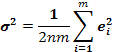
            The quantity used to denote the likely error is called the standard deviation and is given the symbol s. If a large number, N, of readings are taken, and the error made in the i-th reading is e_i, then the square of the standard deviation ( sometimes called the variance ) is given by the equation

            The second type of error listed above, which will be called the tolerance error, is the error due to the coarseness of the scale used. For example, the error made if the scale is read to the nearest 5° may be anything up to 2½° either way. The tolerance error is equally likely to be any value inside the tolerance but is certainly not going to be more than the tolerance. This case is easy to deal with and the standard deviation of the tolerance is calculable theoretically. If the scale is read to the nearest 5° the standard deviation turns out to be 1.28°. In general, if the scale used is marked in divisions spaced at a distance a, then the standard deviation of the distribution of tolerance errors is a/3.46.

            The distribution of the first and third types of error, which will be called the position and reading errors respectively, are certainly nearly normal distributions, but it is unnecessary to attribute any particular form to them. The standard deviations of neither are calculable, so that an experimental determination of the total standard deviation must be devised that will distinguish between them. Fortunately, this distinction is facilitated by the very thing that makes it necessary.

            The error made in measuring angles will be the sum of these three errors, assuming no variation in the magnetic field. In this case the general theory of stochastic processes gives that the standard deviations add in the squares. That is to say, if the standard deviation of the position error, the tolerance error, and the reading error are s_p, s_t, & s_r respectively, then the standard deviation, s, of the total error is given by

            Now s_r and s_t are independent of the distance, d, between the compass and the sighting object, but s_p, the error due to the misplacing of the compass and the sighting object can be written as a/d where a is some quantity independent of d. Thus

Since s_t can be calculated, if s is measured experimentally for two or more values of d, both s_r and a may be individually calculated.

            Objections can be raised to the simple device of setting up a compass and sighting object, taking the bearing of the latter from the former many times, and evaluating s from equation ( 1 ) subsequently. Were this done the same reading would be recorded each time, and, taking the true value of the bearing as the average of all the readings, s would turn out to be zero. This does not point to the failure of equation ( 1 ) but rather to the fact that the errors in such a procedure are not random. Indeed they are not, each being just the same as the other.

            Four points must be borne in mind when devising the experiment to measure o :

            1) the reading recorded in any particular case may be biased by a memory of previous readings if the same or nearly the same angle is measured twice.

            2) it should be certain that the tolerance error really is random in the way indicated above.

            3) it should also be certain that the position error is random, neither this nor the last error will be random if the compass or the sighting object is not continually moved during the experiment.

            4) equation ( 1 ) is true only after an infinite number of readings have been taken. An error is introduced because only a finite number readings can be taken. If the true value of the reading is not known this error enters twice, as the true value has to be taken as the average of all the readings.

            The experiment to be described here takes account of the fourth difficulty while overcoming the first three. Basically, it comprises measurement of the internal angles of an n-sided polygon with a compass and comparing their sum with the known result. The only drawback is that the number of readings that has to be taken to achieve a given accuracy increases by a factor of 2n.

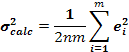
            If there are m polygons each with n sides, and the error in measuring the sum of the internal angles of the i-th polygon is e_i, then the standard deviation, o, is calculated from the formula

The answer obtained for s will be accurate to within 100/ of the actual value ( that value would be obtained if an infinite number of polygons were used ). These two results are derived in the appendix.

            Certain form should be observed during the experiment in order to ensure that reliable answers are obtained. Clearly, since s varies with the distance d, all the sides of the polygons should be the same to within a very few inches. The most suitable polygon to use is a regular pentagon, in the case of three and four-sided figures there would be noticeable similarities between the readings and this would detract from the reliability of the answers. Some order of reading the bearings should be used that introduces the maximum confusion into the memory of previous readings.

            The method of working out the sum of the internal angles is important. Each angle should be evaluated separately as the difference between the forward and back bearings at each point, these angles then being summed. If a different method is used, much of the information from the experiment could be unwittingly thrown away. This method also minimises the effects of magnetic field variation.

            The procedure is then as follows. First stake out a large number of pentagons with a given length of side and evaluate s for that value of d from equation ( 2 ). Then repeat this for at least one more value of d. From the formula

 ,

s_r and a may easily be calculated. s_t is given by:

 ,

where t is the tolerance ( e.g. 1° if readings are taken to the nearest degree).

Appendix

             If the standard deviation on the error of a single reading is s and the standard deviation on the error of the sum of the internal angles of an n-sided polygon is s_t, then, as the sum of the internal angles is an algebraic sum of 2n separate readings,

 ,

            If the error on the sum of the internal angles of the i-th polygon is e_i, then

 ,

so that

 ,

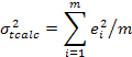
Define s_calc and s_tcalc by the equations

and

Then

Now the probability density of getting an error e_i for the i-th polygon is P_e( e_i ), where

If f_i =  and the distribution of the f_i goes as Pf( f_i ) then

It should be noted here that it is not necessary to assume that either the position error or the reading error follows a normal distribution. The error on one reading follows a distribution that is certainly not Gaussian but the distribution of e_i is the convolution of ten such distributions which are all similar so that it is very close to a normal distribution.

The standard deviation of P_f may easily be calculated by the usual formula and it turns out to be ( = ). The standard deviation of the sum  ( ) is then clearly  so that the standard deviation of the distribution of the quantity   is . It is now easy to see that the standard deviation of the quantity s_calc is about .

The . is the likely error that will be made in measuring s if m polygons are used.

H. I. Ralph,
St. John’s College,
OXFORD.